ODF Matching through the use of Matlab's FMINCON

Problem Definition

The goal of this work is to select a set of less than 5000 orientations and to determine the volume fractions of these orientations required to match an experimental Orientation Distribution Function (ODF) (calculated from a EBSD map from a titanium alloy microstructure). We want to,

$\begin{equation} {minimize}_{v_i} \big\{\sum\limits_{l=0}^\hat{L} \big(\tilde{C}^L - \sum\limits_{i=1}^{N}v_iC_i^L\big)^2\big\} \end{equation}$

where $ \tilde{C}^L $ is the set of reference GSH coefficients (from the experimental ODF), $ C_i^L $ the set of GSH coefficients use to represent the single crystal ODFs in GSH functions and $ L $ permutes $ l $, $\mu $ and $ \nu $.

The following conditions must be imposed to constrain the solution:

$\begin{equation} \sum\limits_{i=1}^N v_i = 1 \end{equation}$ $\begin{equation} 0 \leq v_i \leq 1 \end{equation}$

Optimization Using FMINCON

The following equation is minimized using Matlab’s FMINCON

f = @(V) sum(conj(Y_coeff - X_coeff*V).*(Y_coeff - X_coeff*V) );
[x,fval,exitflag,output] = fmincon(f,Vo,[],[],Aeq,beq,lb,ub,[],options);

$ Y_{coeff} $: The set of GSH coefficients from the OIM software representing the actual ODF
$ X_{coeff} $: An array of GSH coefficients for each selected orientation which have been properly scaled (details are shown in the next section)
$ V $ : Vector of volume fractions associated with each selected orientation

The constraints on the solution were imposed as shown in the following Matlab code:

% an initial guess for the volume fractions of each orientation
Vo = (1/size(X_coeff,2))*ones(size(X_coeff,2),1);
% Aeq * x = beq
Aeq = ones(size(X_coeff,2),size(X_coeff,2));
beq = ones(size(X_coeff,2),1);
% lb =< x <= ub
lb = zeros(size(X_coeff,2),1);
ub = ones(size(X_coeff,2),1);

Development of $ X_{coeff} $

First, the constant $ K $ is defined as

$\begin{equation} K = \frac{e^{-0.25l^{2}w^{2}} - e^{-.25(l+1)^{2}w^{2}}}{1 - e^{ -0.25w^{2}} } \end{equation}$

where $ w $ is the gaussian half-width and is set to 5 degrees

Finally,

$\begin{equation} C_i^{l\mu\nu} = (2l + 1)\sum\limits_{i=1}^N K\dot{\ddot{T}}_l^{\mu\nu}(g_i) \end{equation}$

$ X_{coeff} $ is created by assembling an array of the coefficients where each column is the set of $ C_i^{l\mu\nu} $ indexed by $ i $.

Preliminary Results

The preceding algorithm was employed to approximate the experimental ODF using a set of 360 unique crystal orientations.

Selection of Orientations

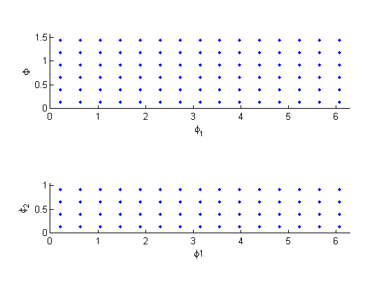
Orientations selected from Hexagonal-Triclinic fundamental zone ($ 0 \leq \phi_1 \leq 2\pi, 0 \leq \Phi < \frac{\pi}{2}, 0 \leq \phi_2 \leq \frac{\pi}{3} $)
The fundamental zone was uniformly binned and a single orientation was selected from the center of each bin for a total of 360 orientations.
- Bin spacing in $ \phi_1 = 24 $ degrees
- Bin spacing in $ \Phi = 15 $ degrees
- Bin spacing in $ \phi_2 = 12 $ degrees

The image below shows the unique orientations selected from the hexagonal - triclinic fundamental zone

Selection of Coefficients to be used in the Optimization

A truncation level of $ L = 7 $ in the GSH functions was chosen to balance the resolution of the answer with the total number of coefficients required (the total number of coefficients at this truncation level is 56). Next, the 0th coefficient and the redundancies in the GSH coefficients were removed, leaving a final set of 30 coefficients for each ODF representation.

Pole Figure Comparison

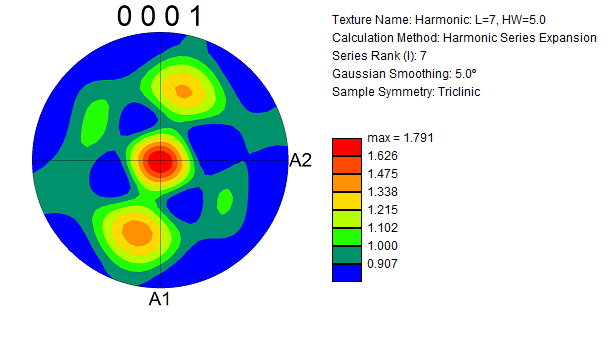
In order to appreciate the quality of the fit, pole figures from the ODF matching were compared to those from the experimental ODF (Pole figures for the ODF matching results were generated by seeding an OIM .ang file with representative volume fractions of orientation readings based on the optimization and running the .ang file through the OIM ODF generation procedure).

The following pole figure is from the ODF matching effort

The following pole figure is from the experimental ODF

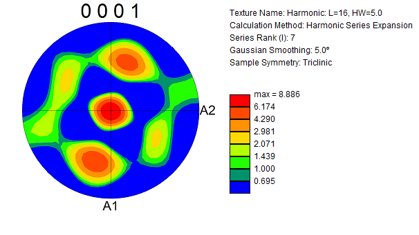
While the qualitative trends in the figures are the same, the intensity at the peaks in the experimental pole figure is greater than those from in ODF matching by an order of magnitude.