Nanoindentation Automated Analysis Example

We have defined some metrics for good analyses previously post. This method still requires some manual selection to remove clusters of analyses that produce bad analyses.

Baseline Analysis

segment size (10:5:400)
overlap requirement low (>10%)
R2 for zero point low (>0.5)
Modulus must be real
No judgment on quality of stress-strain curve

Analysis Work Flow

iterate through segments with the three linear fits saving only necessary variables for filtering
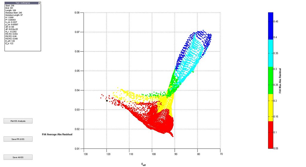
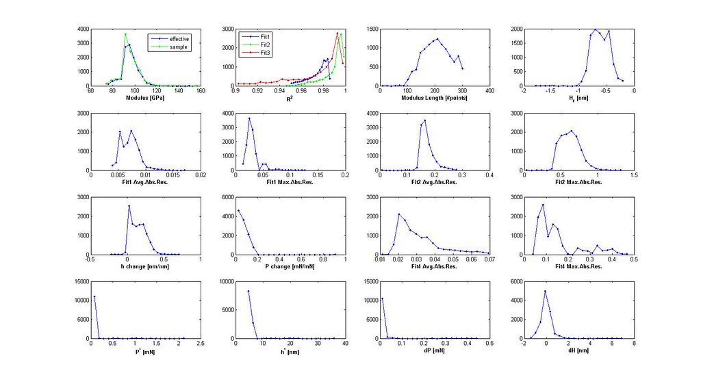
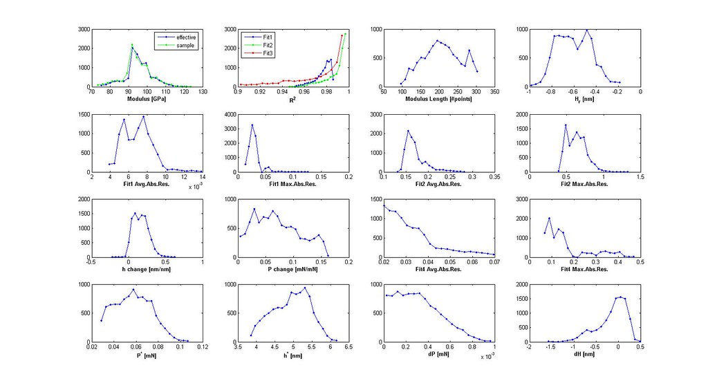
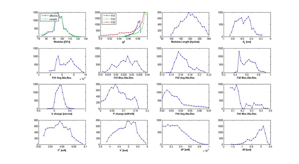
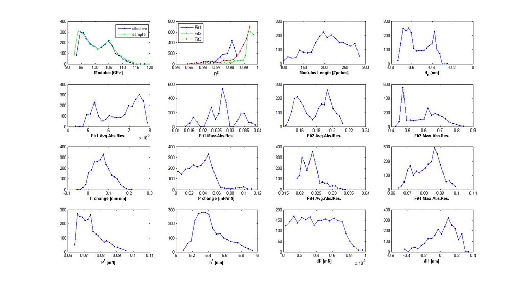
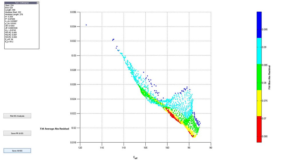
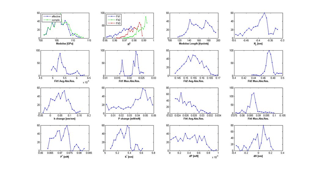
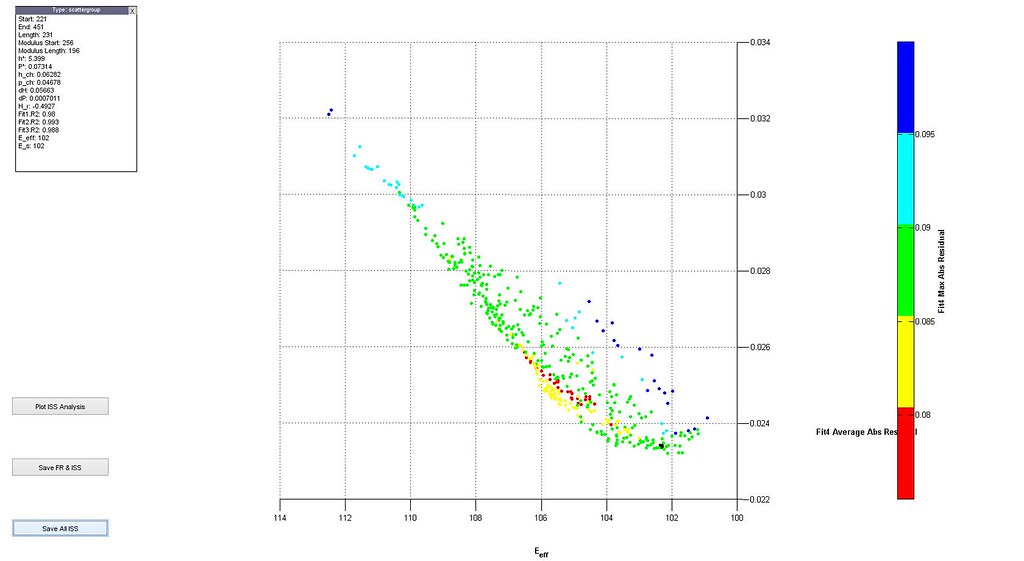
plot distributions 3D scatter plot of filtered analyses
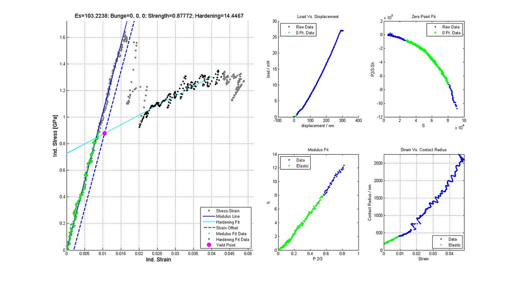
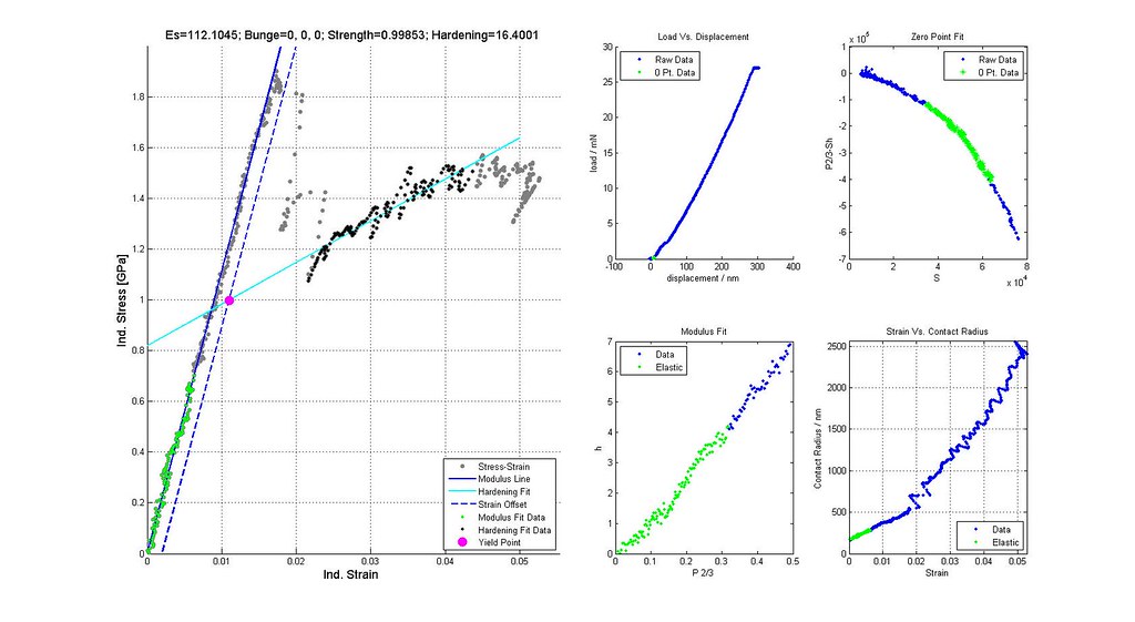
plot stress-strain curves of a few selected analyses particularly at the boundaries of the scatter plot
iterate through filtering using the distributions and 3D scatter plot to determine cutoffs until the majority of the stress-strain curves are acceptable
calculate stress-strain and plastic properties for all acceptable analyses
verify yield strengths are correctly determined from offset or back extrapolated
calculate the statistics of the modulus, yield strength, and hardening
save work space

Case Study

Sample is CPTi, 16um indenter radius, 2014-02-26 Batch #00002. 892 data points. 32,378 Analyses.

Iteration 1

Filt ={ 'Modulus', [1000 10]}

Iteration 2

Filt ={ 'Modulus', [1000 10]; 'R21', 0.95; 'R22', 0.90; 'R23', 0.90}

Iteration 3

Filt ={ 'Modulus', [1000 10]; 'R21', 0.95; 'R22', 0.90; 'R23', 0.90; 'P*', 0.1100}

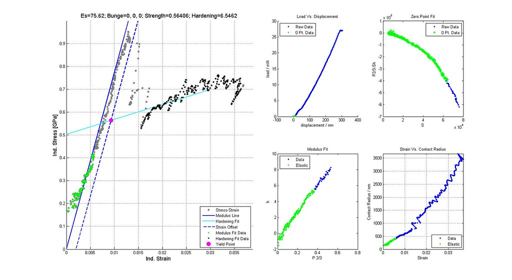
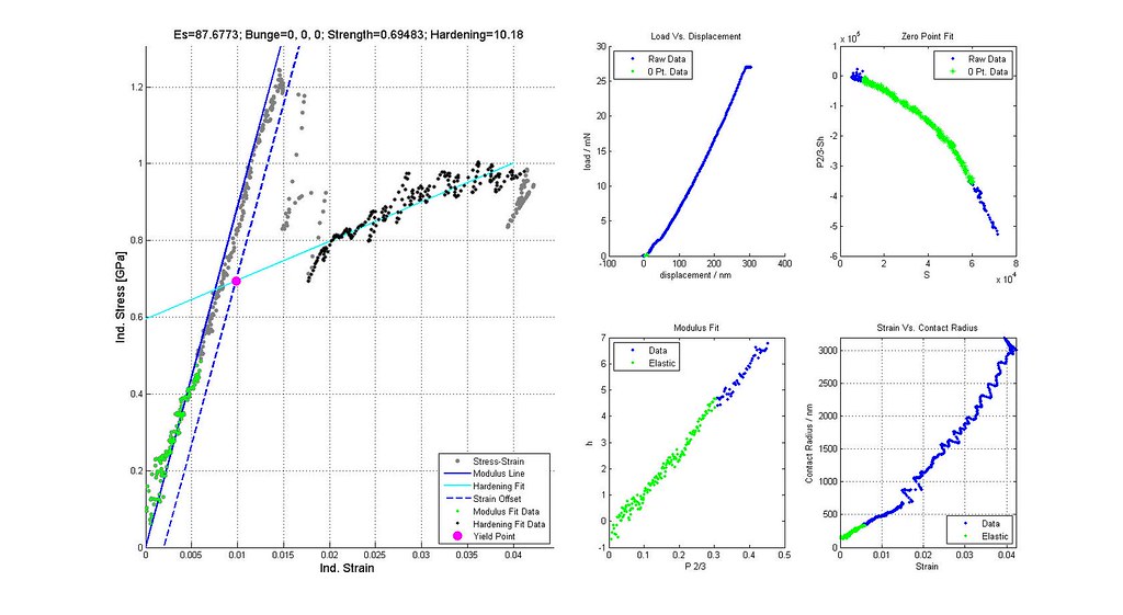
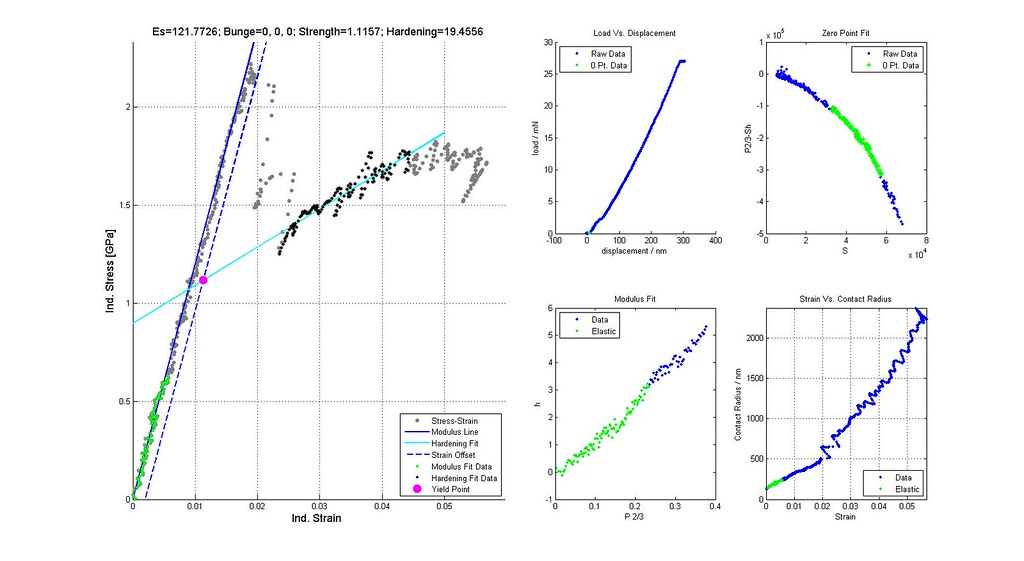
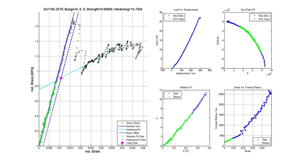
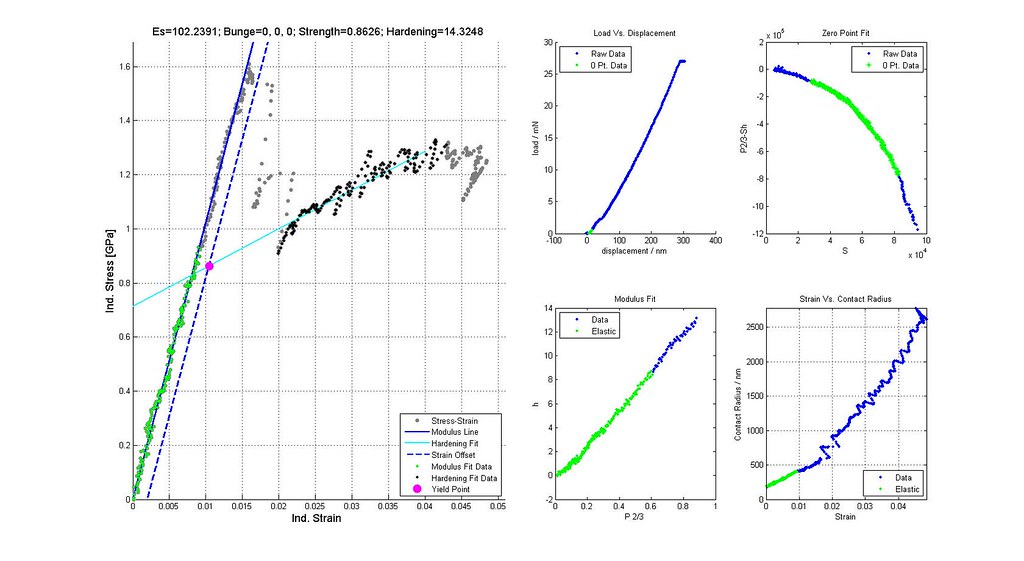
Saved Search Scatter Plot and Example Stress-Strain Curves

Iteration 4

Filt ={ 'Modulus', [1000 10]; 'R21', 0.95; 'R22', 0.90; 'R23', 0.90; 'P*', 0.1100; 'dP', 0.001}

Iteration 5

Filt ={ 'Modulus', [1000 10]; 'R21', 0.95; 'R22', 0.90; 'R23', 0.90; 'P*', 0.1100; 'dP', 0.001; 'MAR1', 0.04}

Iteration 6

Filt ={ 'Modulus', [1000 10]; 'R21', 0.95; 'R22', 0.90; 'R23', 0.90; 'P*', 0.1100; 'dP', 0.001; 'MAR1', 0.04; 'MAR4', 0.1}

Iteration 7

Filt ={ 'Modulus', [1000 10]; 'R21', 0.95; 'R22', 0.90; 'R23', 0.90; 'P*', 0.1100; 'dP', 0.001; 'MAR1', 0.04; 'MAR4', 0.1; 'p_change', [0.06 0]}

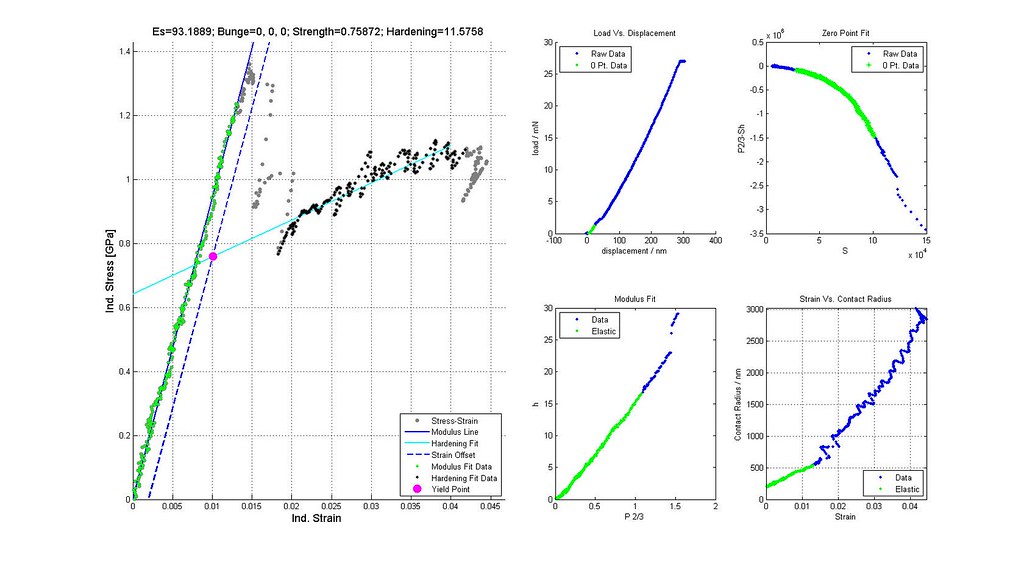
Saved Search Scatter Plot and Example Stress-Strain Curves

Saved all Stress-Strain Data

Estat = 
  mean: 100.0200
median: 99.2786
 stdev: 4.6270
   min: 92.4900
   max: 118.6119

Ystat = 
  mean: 0.8365
median: 0.8220
 stdev: 0.0610
   min: 0.7394
   max: 1.0960

Hstat = 
  mean: 13.4397
median: 13.3776
 stdev: 1.4401
   min: 11.1772
   max: 19.1546

Iteration 8

Filt ={ 'Modulus', [1000 10]; 'R21', 0.95; 'R22', 0.90; 'R23', 0.90; 'P*', 0.1100; 'dP', 0.001; 'MAR1', 0.04; 'MAR4', 0.1; 'p_change', [0.06 0]; 'MAR2', 0.5}

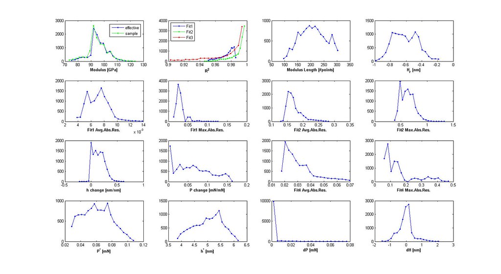
Iteration 9

Filt ={ 'Modulus', [1000 10]; 'R21', 0.95; 'R22', 0.90; 'R23', 0.90; 'P*', 0.1100; 'dP', 0.001; 'MAR1', 0.04; 'MAR4', 0.1; 'p_change', [0.06 0]; 'MAR2', 0.5; 'Hr', [-0.3 -0.5]}

Saved Search Scatter Plot and Example Stress-Strain Curves

Saved all Stress-Strain Data

Estat = 
  mean: 105.8270
median: 105.7222
 stdev: 2.2997
   min: 100.9116
   max: 112.5039

Ystat = 
  mean: 0.9153
median: 0.9173
 stdev: 0.0325
   min: 0.8437
   max: 1.0199

Hstat = 
  mean: 15.1464
median: 14.9451
 stdev: 0.6875
   min: 13.9577
   max: 16.6392

Iteration 10

Filt ={ 'Modulus', [1000 10]; 'R21', 0.95; 'R22', 0.90; 'R23', 0.90; 'P*', 0.1100; 'dP', 0.001; 'MAR1', 0.04; 'MAR4', 0.09; 'p_change', [0.06 0]; 'MAR2', 0.49}

Saved all Stress-Strain Data

Estat = 
  mean: 105.2801
median: 105.5839
 stdev: 2.4332
   min: 99.7603
   max: 110.0666

Ystat = 
  mean: 0.9071
median: 0.9156
 stdev: 0.0338
   min: 0.8320
   max: 0.9784

Hstat = 
  mean: 15.0195
median: 14.8722
 stdev: 0.7281
   min: 13.4207
   max: 16.2188

Progression of number of good analyses based on Filt variables for 10th iteration of Filt.

There is not much more reasoning in filtering the data further

note: Images labeled 6 and 8 are actually for iterations 7 and 9 and correctly positioned in this post. The orientation of the grain where the indent was run is not (0,0,0)

The matlab code and data used for this analysis can be found here: code and data