Spectral Interpolation - Examples in 1D and 2D
Introduction
The Discrete Fourier Transform (DFT) is critical to numerous applications in technology and science. One example is the representation of sophisticated functional relationships in multiple dimensions. Sometimes phenomena are too complex to be described by simple formulae. In these cases one option is to build a database of inputs and associated outputs. Unfortunately, in many cases the domain of possible inputs is extremely large. Many databases end up using substantial memory, yet are too sparse to allow for effective interpolation between values. The advantages of DFTs in such a situation are two-fold:
A. The number of significant frequencies in the DFT is often a small fraction of the total number of frequencies. Therefore, the memory footprint of the representation can be greatly reduced by storing only these critical frequencies.
B. We can interpolate between values in the original database with computational ease by zero-padding in frequency space. This technique is called spectral interpolation.
This post describes spectral interpolation and gives examples of its use in 1 and 2 dimensions. Interpolation in real space generally relies upon linear or higher-order polynomial fits, while spectral interpolation is performed in frequency space with sines and cosines.
1-D Interpolation
Imagine that we start with 16 evenly spaced samples of the function shown below, but we don’t actually know the function itself. In Figure 1 below, the blue line is while the green circles represent the sampled values of the function.

Figure 1
What can we do if we want to know the value of at locations between the sampled values? One option would be to use linear interpolation between 2 sampled data points. This is fine, but since isn’t linear this will introduce error. Higher order polynomial fits are an option, but these become computationally expensive to compute. Spectral interpolation is advantageous because it allows us to “fill in” between the original sampled values and do so for the entire domain of the function through a single computation.
The first step in spectral interpolation is to take the DFT of the samples using a FFT algorithm. Through this technique we represent the function in frequency space, where each frequency contains information about the amplitude and phase shift of the associated sinusoid. The following image shows the real and imaginary components of the frequencies of the DFT. Notice the symmetry in both real and imaginary components.
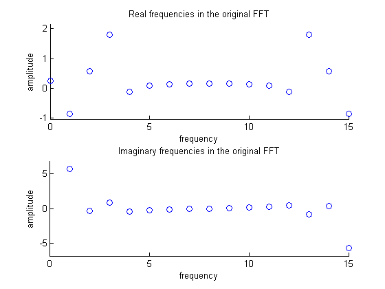
Figure 2
The key to spectral interpolation is “zero-padding.” By inserting zeros into the DFT at a specific location the number of frequencies is increased. Since the number of samples in real space matches the number of frequencies in the DFT, zero padding in frequency space increases the number of values in real space as well. So long as the function was sufficiently sampled in real space, spectral interpolation approximates the intermediate values with arbitrary precision.
Due to the symmetry inherent in the DFT representation, we split the spectrum in half and insert zeros at the center (these represent higher frequencies with no contribution to the representation). The following image shows the real and imaginary components of the DFT after zero padding.
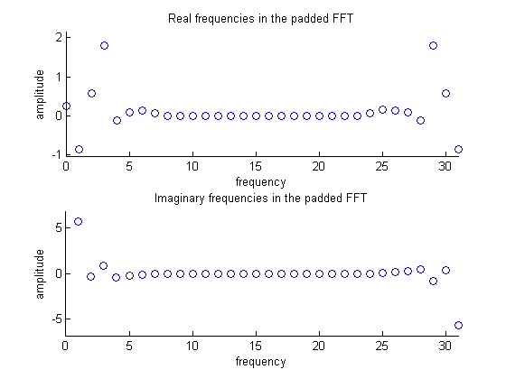
Figure 3
Finally, the inverse FFT is taken and the result is scaled by the ratio of the number of frequencies in the zero-padded DFT to the original DFT. Through this method we interpolated between our sampled values (see the red crosses in Figure 1) in a way that closely matches the original function.
Side Notes:
-
The function is periodic over the domain . If were not periodic the DFT method would be less effective, as the DFT assumes periodicity. In this case we would mirror the function over the vertical axis (to make it periodic over the domain and of at least continuity).
-
To calculate the interpolated value of at a single location simply perform the inverse DFT for a single location in real space. This is important when the original database is large or precise interpolation is desired.
2-D Interpolation
In this case we start with a function with 2 inputs. Spectral interpolation works much in the same way as for the 1D case.
The original function is as follows:
As before we sample the function at regular intervals and perform the DFT using the FFT algorithm. As the input data is now 2-D the FFT is performed on one axis first and then on the other (the order doesn’t matter).
The major difference with the 1-D case is in the insertion of zeros into the DFT. The zero padding scheme is visually demonstrated below in Figure 4.
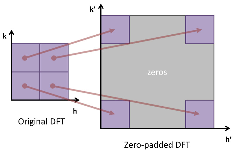
Figure 4
Again, the inverse FFT is performed and the result is scaled by the ratio of the number of frequencies in the zero-padded DFT to the original DFT. As shown in Figure 5, was effective in interpolating between the sampled values in 2 dimensions.
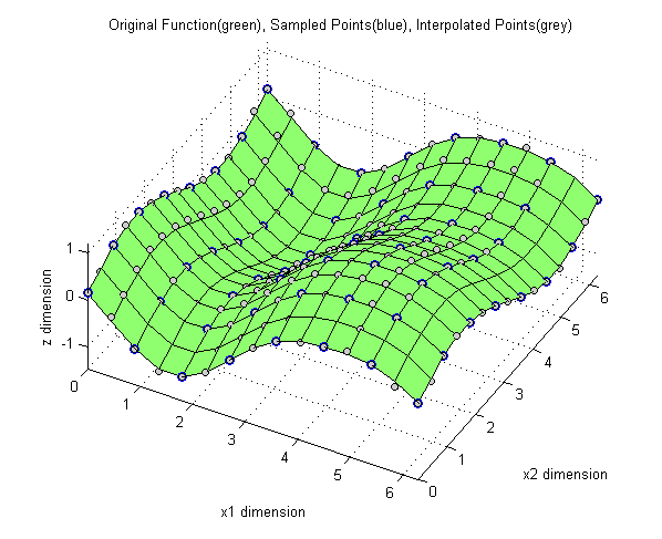
Figure 5
References
-
For another easy introduction to spectral interpolation see the following link.
-
R.G. Lyons Understanding Digital Signal Processing 3rd edl. 2010 Prentice Hall
-
B.L. Adams, S.R. Kalidindi, D.L. Fullwood Microstructure Sensitive Design for Performance Optimization 2012 Butterworth-Heinemann