NISSAA Code Structure
-
This post is an outline of the structure of the NanoIndentation Stress-Strain Analysis Automation (NISSAA) code written in Matlab. It is meant to help users run, debug, and augment the code.
-
This code is an experiment: can the zero point correction and indentation stress-strain curve be objectively determined and automated by using a limited number of metrics to sort through all possible solutions?
-
The original details of the analysis can be found in Kalidindi, S.R. and S. Pathak. “Determination of the effective zero-point and the extraction of spherical nanoindentation stress–strain curves.” Acta Materialia. 2008.
-
Scroll to the bottom for relevant links
RunMe.m
RunMe.m contains most relevant variables which the user will need to change and calls three main fucntions: Driver.m, SearchExplorer.m, and MyHistResults.m. It first calls the function Driver.m and outputs structures TestData and FitResults
Variables
- file and sheet are used to specify the location of the raw data in excel
- seg_sizes is an array of segment sizes used to generate analyses
- Rind is the indenter radius in nanometers
- vs is the sample Poisson ratio used in calculating the sample modulus
- skip is a two value array which allows you to skip or not record analyses which have r-squared values less than skip(1) in the zero point linear regression OR a segment length ratio (the number of data points used in the effective modulus linear regression over the number of data points in the zero point linear regression) less than skip(2)
1. Driver.m
Calls LoadTest.m and SingleSearchResults.m
1.1 LoadTest.m
In here you may need to change the indenter properties if not diamond (Ei and nus), what test segment you want to stop at (currently ‘Unloading Marker’), and what columns to load.
T = num(1:HoldSegmentII, 1:6); % Takes the first 6 columns with numeric values
1.2 SingleSearchAllSegments.m
In here NIAnalyzeSearch.m is called over and over marching through the test data one point at a time for each segment size input.
1.2.1 NIAnalyzeSearch.m
Here is where the zero point and effective modulus fit regressions are performed along with many other calculations which help to decide if the analysis is good (this decision comes later with the exception of skip which ends the analysis on the spot). NIAnalyzeSearch.m calls rsquare.m, mypolyfit.m, polyval, etc for linear fits.
Variables (limited set)
- segment_start staring point of zero point linear regression (Fit1)
- segment_end end point of Fit1
- segment_length is the number of data points in Fit1
- modulus_start start point for effective modulus linear regression (Fit2)
- modulus_end does not exist because it is the same value as segment_end
- modulus_length is the number of data points in Fit2
- h_star is the displacement zero point correction
- P_star is the load zero point correction
- h_change is the ratio of the difference of Fit2 displacements (end - start) and Fit1 displacements (end - start)
- p_change same as above but with loads
- dH is the value of the zero point corrected displacement at the start of Fit2
- dP same as above but for load
- E_star is the effective modulus
- Fit3 is a structure for a linear fit to the stress-strain data for the same range in Fit2.
- Fit4 is a structure for an error calculation between the effective modulus line plotting starting at the origin of the stress-strain plot and the data for the same range in Fit2.
Each Fit# (1,2,3,4) has three metrics to determine the goodness of fit
- R2# r-squared value (not for Fit4)
- AAR# average absolute residual
- MAR# maximum absolute residual
2. SearchExplorer.m
Once FitResults is generated RunMe.m next calls SearchExplorer.m. Here we will filter the results to ones of interest and plot them in a 3D scatter plot with a colormap which allows for a selection of four parameters. The outputs of SearchExplorer.m are SearchResults which contains all the FitResults that survived the filter operations, npoints which catalogs how many analyses remain after each filter operation, and HistSearchResults which are histogram values for select variables for the FitResults that survive the filter operations. A multi histogram plot of these results is also performed.
Helpful Note: Generating FitResult from Driver.m is a one time event (that takes the most time to run) unless you decide to change some of the variables that went into Driver.m. You can iterate through filtering and plotting by just rerunning SearchExplorer.m !
Variables (inputs to SearchExplorer.m)
- Filt is a cell array with a string and vector. The list of strings is as follows
- ‘Modulus’ filters based on effective modulus
- ‘R21’, ‘R22’, ‘R23’- rsquared of Fit1, Fit2, and Fit3
- ‘P*’ filters based on the zero point load correction
- ‘h*’ same as above for the zero point displacement correction
- ‘dP’ filters based on the dP
- ‘dH’ same as above for dH only
- ‘p_change’ filters based on p_change
- ‘h_change’ same as above for h_change
- ‘ModLength’ filters based on the number of data points in Fit2
- ‘AAR#’ filters based on the average absolute residual for the Fit#
- ‘MAR#’ filters based on the average absolute residual for the Fit#
- ‘Hr’ filters based on the y-intercept of Fit2 (residual height)
One to all the strings can be used in Filt, and the order is not important for the final number of analyses kept. However if you want to know how many analyses are discarded for each filter, the order is important as the discarding happens sequentially from the first to the last string. The filtering is done in filterResults.m, and any new variable can be easily added by adding another case.
- bins is the number of bins used in the histogram plots
- Plastic is a structure containing most relevant variables for determining the yield strength and hardening
- YS_offset is the offset strain for determining the YS using a modulus offset line
- H_offset is the offset strain using a modulus line that bounds the Hardness slope determination
- pop_in is the minimum change in strain for pop_window that IDs a pop_in event which then requires the back extrapolation method for determining yield strength. If no pop-in is detected, the strain offset method is used for determining yield strength.
- pop_window is the number of points used to calculate the change in strain i.e.
- C_dstrain is a fudge factor used for the start of the hardening slope and back extrapolation fit that eliminates the high sloped region in the shadow of a pop-in. A value of 1 would skip all the data in the shadow of the pop-in. A value of 0 would start the fit at the full unloading point of the pop-in.
- YS_window is the percent to the left and right of YS_offset used for calculating the yield strength when no pop-in is detected (i.e 0.30 would make a window 0.7 and 1.30 around YS offset)
- smooth_window is the number of data points used for a moving average (i.e. 10 points before and 10 points after) on strain before the hardening and back extrapolation fits are performed. This is done in smoothstrain.m.
Most of the variables in Plastic are used in FindYieldStart.m and FindYield.m
- BEuler is an array for the three Bunge-Euler angles for crystalline materials only used for archiving and display on plots.
2.A The 3D scatter plot plus colormap
Here is an example of the plot. A data point is single analysis. Clicking on a point will generate a window with a list of values for that analysis. The 3D plot can be rotated for easier viewing. The plot also contains three buttons which perform actions.
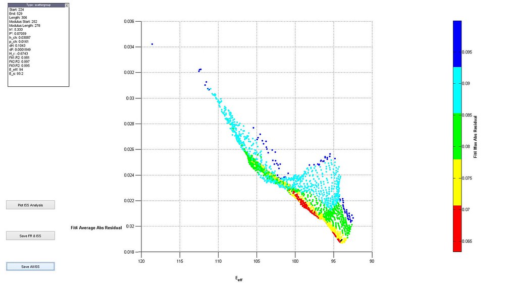
1.2.A.1 Plot ISS Analysis allows you to perform and plot the indentation stress-strain analysis for the selected single analysis. An example plot is shown below.

1.2.A.2 Save FR & ISS allows you to save the FitResults and Stress-strain analysis in a structure called Stress Strain Analysis for the selected single analysis. 1.2.A.3 Save All ISS saves all the stress-strain analyses associated with SearchResults in a structure called Stress Strain Search Results.
Helpful Note: If you want to change the variables in the 3D plot you have to change code in two places.
In SearchExplorer.m
index = find(p(1) == [Fit4.AverageAbsoluteResidual] & p(2) == [FR.E_star] & p(3) == [FR.h_change], 1, 'first');
In MyPlotSearch.m
h = scatter3([Fit4.AverageAbsoluteResidual], [SearchResults.E_star], [SearchResults.h_change],10, [Fit4.MaxAbsoluteResidual], 'filled');
2.1 MyPlotSearch.m
In here is where filterResults.m is called and the 3D scatter plot is made. See the explanation for Filt for more details of filterResults.m.
2.2 CalcStressStrainWithYield.m
This function calculates and records stress, strain, yield strength, and hardening into a structure.
2.2.1 FindYieldStart.m
This determines if a pop-in occurred and finds the starting and end points for the hardening or back extrapolation fit. The starting point is found by two different methods: strain offset or the minimum stress of the data after a pop-in is identified (with a fudge factors, see Cdstrain).
- Strain offset method for the starting point is the intersection of the offset line (see YS_offset) with the stress-strain curve.
- Minimum stress method is only used when a pop-in is identified and finds the minimum stress after the pop-in and moves slightly further along depending on the value of Cdstrain.
The end point is found the same way regardless of a pop-in. A strain offset line is used to find the intersection with the stress-strain curve (see H_offset). If there is not enough data, the last point is used within the limits of the smooth window value (i.e. last point - smooth window).
2.2.2 FindYield.m
Here is where the yield strength and hardening are determined. There are two methods to calculate the yield strength: the median of an offset strain window or a back extrapolation.
- Median of an offset strain window is used when no pop-in is detected. The offset strain window determined from YS window is about the offset strain from YS offset. The median of all the stress values within this window is the yield strength. Using reduces the influence of noise in the curve on the yield strength.
- The back extrapolation method is used when a pop-in is detected. A linear fit to the stress-strain data is performed between the start and end points determined in FindYieldStart.m. The intersection of this line and the offset line from YS offset is the yield strength.
The hardening is simply the linear approximated slope of the stress-strain curve between the start and end points determined in FindYieldStart.m. Note that a moving average is used (see smooth window and smoothStrian.m). Also the starting point is determined from two different methods as outlined above for FindYieldStart.m. If the back extrapolation method is used, this fit is also the hardening fit.
Helpful Note: The variable popin YN indicates whether a pop-in was detected: 0=yes, 1=no. The variable fullH YN indicates if there was enough stress-strain data to reach the H offset line: 0=yes, 1=no.
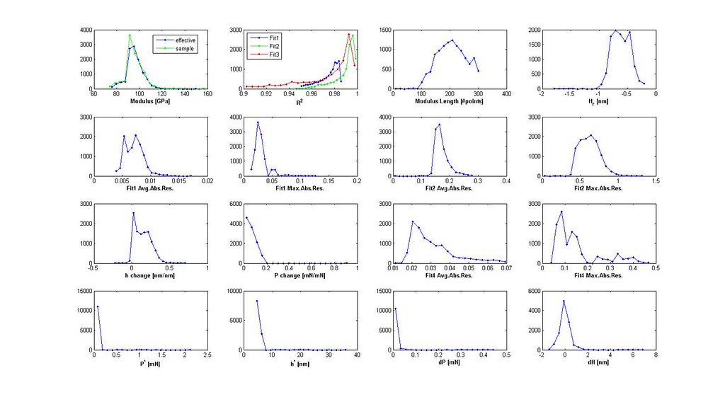
2.B The Historgram Plot
The histogram plot is generated through MyHistSearch.m. See bins for setting the number of bins in the histogram plot. An example is shown below for 16 different parameters. You can use the histograms to decide on Filt selections and values.
3. MyHistResults.m
Run this function when you are finished filtering out poor analyses and want to compute some simple statistics on the remaining analyses. This will calculate the mean, median, standard deviation, and min and max values for the sample modulus, indentation yield strength, and indentation hardening. You can add more variables as desired with some simple modifications. Here is a sample output
Estat =

  mean: 109.1988
  median: 109.7483
  stdev: 7.2921
  min: 96.5710
  max: 120.8406


Ystat =

  mean: 0.9411
  median: 0.9566
  stdev: 0.0877
  min: 0.7862
  max: 1.0795


Hstat =

  mean: 18.3343
  median: 18.0011
  stdev: 2.1059
  min: 14.9636
  max: 21.8466
Saving Your Workspace
I recommend saving your workspace as a .m file for each test. You can load your workspace at a later date, change any of the variables, and rerun one or all three of the functions above. For this you should make a modified RunMe.m file so that you don’t overwrite the parameters in your workspace you don’t want to change or just work from the command window to call the three main functions.
Code
- The latest NISSA code written in Matlab can be accessed here.
- Please note that CSM corrections are applied to the data before doing any linear regressions. See this post CSM corrections for reasons why.
- Also note that the indentation strain is the sample strain which comes from correcting the total displacement for the indenter tip displacement. See this post Sample Strain for a full explanation.
- See these posts theory and example for some explanation on how to filter results (for an older version of code, but the ideas are the same).
Many thanks to David Turner and Shraddha Vachhani for starting this effort and Calvin Miller for his semester of work adding to it.